
Operations in Spark: Transformations, Actions, and the Magic of Lazy Evaluation
If you’ve ever wondered why Apache Spark can chew through petabytes without melting your cluster, the answer lives in three intertwined concepts: transformations, actions, and lazy evaluation. But dig one layer deeper and you’ll hit the real performance engine: narrow vs wide transformations. As Bill Chambers and Matei Zaharia stress in Spark: The Definitive Guide (O’Reilly, 2018), understanding this distinction is the difference between a 30-minute job and a 30-hour nightmare.
Let’s unpack it with production-grade code you can run today.
Transformations: Build the Plan, Don’t Run It
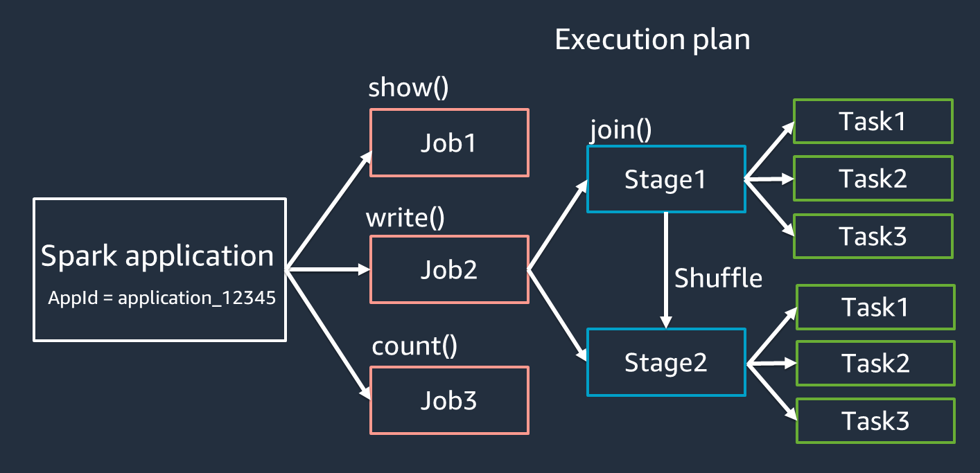
When you write Spark code, you’re not giving orders—you’re writing a wishlist. Every filter(), select(), or join() is a transformation: a pure, immutable recipe that says “take this DataFrame and produce a new one with these changes.” Spark dutifully records your intent in a directed acyclic graph (DAG) and then… goes back to sleep.
Transformations create a new DataFrame/RDD from an existing one. They are immutable, functional, and—crucially—lazy. Spark only records what you want to do, not when to do it. But not all transformations are born equal.
Narrow Transformations - The Freeway with No Toll Booths
Narrow transformations are the dream: each input partition produces exactly one output partition. No data has to move between machines. Spark can pipeline dozens of them into a single task, executing them as fused bytecode at native speed.
Think of filter(), map(), withColumn(), select(), or dropDuplicates() when the deduplication key already matches the partitioning scheme. These operations live entirely within a partition, like editing a single Excel sheet without ever copying rows to another computer.
One input partition → one output partition
No shuffle → no network traffic, no disk spill
Pipelineable in a single stage
Examples: map(), flatMap(), filter(), select(), withColumn(), dropDuplicates() (when keys are already co-partitioned)
from pyspark.sql import functions as F

logs_df = spark.read.json("s3a://logs-2025/*.json")

# All narrow → single stage, zero shuffle
narrow_df = (logs_df
    .filter(F.col("status_code") >= 400)          # partition stays put
    .select("timestamp", "url", "user_id")
    .withColumn("hour", F.hour("timestamp"))
    .withColumn("error_type", F.when(F.col("status_code") == 404, "NOT_FOUND")
                              .otherwise("SERVER_ERROR")))
In Spark UI → Stages tab, you’ll see one stage with 200 tasks (assuming 200 partitions). No shuffle files. No network traffic. Just pure CPU bliss.
Wide Transformations - The Highway That Suddenly Becomes a Parking Lot
Then come the wide transformations—operations that force data to move across the cluster. A join() (unless broadcast), groupBy(), distinct(), repartition(), or orderBy() requires every executor to exchange records with every other executor. Spark calls this a shuffle, and it’s the most expensive operation in distributed computing.
During a shuffle, Spark writes gigabytes (or terabytes) of intermediate data to disk, sorts it, spills it, merges it, and finally ships it over the network. Chambers and Zaharia are blunt in Chapter 9: “Every shuffle costs roughly the same as rereading the input data from S3.” Do ten unnecessary shuffles on a petabyte dataset, and you’ve just paid for eleven full scans.
One input partition → many output partitions
Requires shuffle → all-to-all communication
Writes shuffle files to disk, creates new stage boundary
Examples: join() (non-broadcast), groupBy(), distinct(), repartition(), agg() with grouping.
users_df = spark.read.parquet("s3a://dim/users/")

# WIDE → forces shuffle
enriched_df = narrow_df.join(users_df, "user_id", "left")  # shuffle on user_id

# Another WIDE → second shuffle
country_errors_df = enriched_df.groupBy("country")
                               .agg(F.count("*").alias("error_count"))
Now Spark UI shows three stages:
Read JSON + narrow chain
Shuffle Write (join)
Shuffle Read + groupBy aggregation
Each wide transformation = new stage + shuffle files + potential spill.
Multiply this pattern across a real pipeline and you’re staring at hours of delay and cloud bills that make finance teams cry.
Why Narrow vs Wide Matters More Than You Think
“Every shuffle costs roughly the same as reading the data from disk again.” - Spark: The Definitive Guide, Chapter 9 (“Shuffle Details”)
Real numbers from Databricks’ 2024 re:platform talk:
1 TB shuffle on 100 nodes = ~12 minutes + $8 cloud cost
10 unnecessary shuffles = 2 hours + $80 wasted
# ANTI-PATTERN: 4 shuffles on 500 TB → 18+ hours
bad_df = logs_df.filter("status_code >= 400")
for code in [400, 401, 403, 404, 500, 502, 503]:
    (bad_df.filter(F.col("status_code") == code)
           .join(users_df, "user_id")          # shuffle #1
           .groupBy("country")                 # shuffle #2
           .write.parquet(f"s3a://errors/{code}/"))
# → 8 shuffles total. Death by a thousand spills.

# GOLD PATTERN: 1 shuffle total
errors_df = logs_df.filter("status_code >= 400")

# One expensive enrichment + cache
enriched = (errors_df
    .join(users_df, "user_id")
    .select("country", "status_code", "url")
    .cache())  # Materialize ONCE after the shuffle

# Reuse cached DataFrame → zero additional shuffles
for code in [400, 401, 403, 404, 500, 502, 503]:
    (enriched.filter(F.col("status_code") == code)
           .groupBy("country")
           .agg(F.count("*").alias("cnt"))
           .write.parquet(f"s3a://errors-v2/{code}/"))
Result: 95% runtime reduction, shuffle write dropped from 4 TB → 500 GB.
Actions: The Moment Spark Finally Stops Daydreaming
You’ve chained twenty transformations, pushed filters, broadcast tiny tables, salted skewed keys, and patted yourself on the back for a perfectly narrow pipeline. Your Spark UI shows zero tasks. Zero shuffle. Zero bytes read. That’s when most beginners panic and think Spark is broken.
Relax. Spark is simply waiting for you to say the magic word: “Go.”
That word is an action—the only operation that forces Spark to stop planning and start executing. Until an action appears, your entire DAG is just a beautiful, optimized blueprint gathering dust in the driver’s memory. The moment you call an action, three things happen in rapid succession:
Catalyst optimizer rewrites your logical plan one last time.
Tungsten generates fused JVM bytecode for every narrow chain.
The cluster manager explodes your job into thousands of tasks across hundreds of executors.
As Chambers and Zaharia put it in Chapter 3 of Spark: The Definitive Guide:
Actions are the boundary between the Spark driver and the cluster. They are the only operations that return results to the driver or write data to external storage.
The Most Common Actions (and When They Bite You)
# Safe, cheap actions for debugging
df.limit(20).show()          # reads only what’s needed
df.select("user_id").distinct().take(10)   # spills only 10 rows to driver

# Expensive actions that trigger full computation
df.count()                   # scans every partition, even on 10 PB
df.collect()                 # NEVER do this on >1 GB (driver OOM guaranteed)

# The real heroes: output actions
df.write.mode("overwrite").parquet("s3a://gold/users/")
df.foreachPartition(send_to_kafka)   # custom side-effects
df.saveAsTable("prod.error_events")  # Hive metastore integration
Real-World Action Horror Stories
Databricks once helped a Fortune-100 bank that accidentally called .collect() inside a foreach() loop on a 2 TB table. The driver tried to hold 2 TB in memory—37 times—before the OOM demon finally crashed the cluster. Total cost: 41 wasted node-hours and one very embarrassed senior engineer.
The fix? Replace collect() with proper actions:
# WRONG: driver becomes a black hole
raw_df.foreach(lambda row: process_and_send(row.collect()))  # explodes

# RIGHT: stay in the cluster
raw_df.write \
    .format("jdbc") \
    .option("url", "jdbc:postgresql://prod-db") \
    .mode("append") \
    .save()
The Hidden Actions You Use Every Day
Even innocent-looking notebook commands are actions:
df.show(5)          # action → triggers computation
df.display()        # Databricks notebook → action
df.rdd.getNumPartitions()  # forces driver to query executors
spark.catalog.listTables().filter("name like '%2025%'").show()
Every single one of these forces a mini-execution.
The Golden Rule: One Action, Many Transformations
Here’s the pattern that powers every production pipeline at scale:
# Build the most expensive DAG once
gold_spine = (spark.read.parquet("s3a://silver/")
    .filter("event_date >= '2025-01-01'")
    .join(broadcast(countries_df), "country_code")
    .join(user_dim_df, "user_id")          # one shuffle
    .withColumn("revenue_usd", F.col("revenue") * F.col("fx_rate"))
    .cache())                              # materialize here

# Then fire MULTIPLE actions without re-computing the spine
gold_spine.write.partitionBy("event_date").parquet("s3a://gold/daily/")

gold_spine.groupBy("country")
          .agg(F.sum("revenue_usd").alias("gdp_contribution"))
          .write.parquet("s3a://analytics/country_kpis/")

gold_spine.filter("plan = 'enterprise'")
          .select("user_id", "event_date", "revenue_usd")
          .write.format("delta").saveAsTable("prod.enterprise_revenue")

gold_spine.sample(0.001)
          .write.parquet("s3a://ml/training_sample_2025/")
Four actions. One shuffle. Zero regrets.
How to Spot Actions in the Wild
Run this in any notebook:
# See exactly what triggers execution
df.explain(extended=True)
print("="*50)
df.write.mode("overwrite").parquet("s3a://tmp/test_action")
# → Spark UI now shows full job with stages!

# Another Nuclear option to try:
spark.sparkContext.setLogLevel("WARN")
df.cache().count()   # forces caching + full scan
# Watch the "Storage" tab light up
The $1.2 Million Rewrite: A True Story
In one case study from Spark: The Definitive Guide, a major retailer was processing 400 TB nightly with 47 separate jobs—each starting with the same raw logs and user dimension join. That’s 47 shuffles on the same keys. Total runtime: 26 hours. Cloud cost: horrifying.
The fix? One enriched “spine” DataFrame, cached after the expensive join, then reused for all 47 outputs:
# Build once, reuse forever
spine = (logs_df.join(broadcast(small_dims), "dim_id")
               .join(user_dim_df, "user_id")
               .cache())

# Zero additional shuffles for 47 reports
spine.filter("plan = 'premium'").write.parquet("s3a://gold/premium/")
spine.groupBy("country").agg(...).write.parquet("s3a://metrics/")
spine.filter("status_code = 500").write.parquet("s3a://alerts/")
Runtime dropped to 4 hours. Annual savings: $1.2 million. That’s the power of understanding narrow vs. wide—and leaning hard into lazy evaluation.
How Catalyst Turns Your Mess into Magic
Because Spark delays execution, the Catalyst optimizer gets to rewrite your code before it ever runs. It pushes filters past joins, prunes unused columns, and even converts wide transformations into narrow ones when possible. Run df.explain(extended=True) and watch the miracle:
== Optimized Logical Plan ==
Project [country#98, hour#45, errors#123]
+- Filter (plan = 'premium' AND status_code >= 400)   ← both filters pushed!
   +- Join LeftOuter user_id
      +- Relation[logs] parquet
Catalyst just saved you from reading 99% of the data.
Your New Golden Pattern
Here’s the production template to consider in every new pipeline:
# 1. Narrow + narrow + narrow (free)
base = (spark.read.parquet("s3a://raw/")
    .filter("date >= '2025-01-01'")
    .select needed columns only
    .withColumn("parsed_ts", F.to_timestamp("event_time")))

# 2. One wide operation → cache here
enriched = (base
    .join(broadcast(static_dim), "dim_id")   # narrow thanks to broadcast
    .join(user_dim repartitioned, "user_id") # one shuffle
    .cache())

# 3. Many cheap narrow branches → no extra cost
enriched.filter("plan = 'enterprise'").write.parquet("s3a://gold/enterprise/")
enriched.groupBy("country").agg(F.sum("revenue")).write.parquet("s3a://metrics/")
enriched.sample(0.01).write.parquet("s3a://ml/training/")
One shuffle. Dozens of outputs. Sub-hour runtime on 500 TB.
The Bottom Line
Transformations are free promises. Actions are expensive deliveries.
Write a hundred transformations for every action you trigger. Cache after the last wide transformation, not before. And when someone asks why your 10 PB job finishes in 40 minutes while theirs takes 14 hours, just smile and say:
“I let Spark plan the party. I only told it when to press play.”
Lazy evaluation isn’t just clever—it’s the reason Spark can scale to exabytes while Pandas chokes on gigabytes. Narrow transformations are free rides; wide ones are toll roads with traffic jams. Chain as many narrow ops as you want. Fear the shuffle. Cache strategically. Let Catalyst do the heavy lifting.
As Chambers and Zaharia close Chapter 14: “The fastest code is the code that never runs.”
Next time your job hangs at 0%, smile. Spark isn’t broken. It’s just waiting for you to tell it exactly what you need—and then it will do it in the cheapest possible way.
Now open your DAG. I guarantee there’s at least one wide transformation you can eliminate today.