
Structured Streaming Core in Apache Spark: Your First Real-Time Pipeline (2025 Guide)
Imagine writing the exact same DataFrame or SQL code you use for batch jobs… and then telling Spark “run this forever on live data.” That’s exactly what Structured Streaming does. There are no new APIs to learn, no topology diagrams, no custom checkpointing logic. You describe what the final table should look like, pick a source and a sink, hit start, and Spark continuously and fault-tolerantly updates the result as new data lands. Behind the scenes it uses the full Catalyst optimizer, Tungsten execution engine, checkpointing, and write-ahead logs to give you end-to-end exactly-once guarantees — all for free.
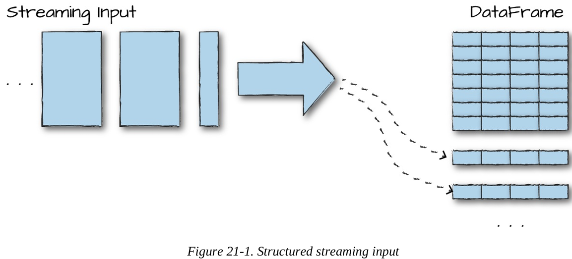
The core mental model is ridiculously simple: a stream is just an unbounded table that keeps growing with new rows. Your query runs continuously against that ever-appending table. That’s it. Everything else (incrementalization, state management, recovery) is handled automatically.
This unification is why thousands of companies now build live dashboards, real-time ETL, fraud detectors, and recommendation systems with nothing more than the DataFrame code they already wrote for yesterday’s batch jobs.
Core Concepts You Actually Need to Know
Structured Streaming keeps the terminology count deliberately low. Here are the only things you’ll ever deal with:
Transformations Almost every DataFrame operation you already know (select, filter, groupBy, join, window, etc.) works unchanged. A few stateful operations had restrictions in very old versions, but in Spark 3.5+ basically everything is supported.
The one and only action There’s no df.show() or df.collect() in streaming. The only action is start() — it launches a long-running query that never stops until you cancel it.
Input Sources (where data comes from) Spark ships production-ready connectors for:
Kafka (0.10+) – by far the most popular
Cloud storage folders (S3, ADLS, GCS, HDFS) – auto-discovers new files
Socket / Rate source – great for tutorials and tests
Many others via the community (Kinesis, Pulsar, MQTT, etc.)
Sinks (where results go)
Kafka
Almost any file format (Parquet, Delta, JSON, CSV, …)
Databases via foreachBatch or JDBC
Console & memory sinks (debugging)
Custom sinks with ForeachWriter
Output Modes (how results are written)
Append – only new rows (perfect for events that will never change)
Update – changed rows only (e.g., updating running totals in a database)
Complete – dump the whole result table every trigger (small aggregations → dashboard)
Triggers (when to process new data)
Default (micro-batch as fast as possible) – lowest latency
Processing-time trigger (e.g., every 5 seconds or 1 minute) – avoids tiny files
Once trigger – for “run exactly once and stop” workloads
Continuous mode trigger (sub-100 ms latency) – available since Spark 3.0
Event Time & Watermarks Event time = the timestamp inside your data (e.g., when the click actually happened), not when Spark saw it. Watermark = “I’m willing to wait maximum 30 minutes for late data.” Once the watermark passes a certain time, Spark knows it’s safe to close windows, evict old state, and emit final results. Without watermarks, state would grow forever.
That’s literally everything you need to understand before writing your first production pipeline. The rest of the chapter (and the next ones) is just showing these concepts in code.
Structured Streaming in Action: Your First Live Pipeline (Hands-On)
Let’s stop talking theory and actually run something. We’ll use the public Heterogeneity Human Activity Recognition dataset – real accelerometer and gyroscope readings from smartphones and smartwatches while people walked, sat, biked, climbed stairs, etc. It’s a perfect example of the never-ending sensor streams you see in IoT, fitness trackers, and industrial monitoring.
You can download the dataset here: https://archive.ics.uci.edu/ml/datasets/Heterogeneity+Activity+Recognition (Just grab the “Activity data” folder – it’s a few hundred JSON files.)
Step 1 – Peek at the data with a normal batch read
# Python / PySpark
static = spark.read.json("/path/to/activity-data/")
static.printSchema()
static.show(5)
Key columns you’ll see:
Arrival_Time – when the record hit the server
Creation_Time – actual device timestamp (nanoseconds!)
Device, Model, User – metadata
gt – ground-truth activity: "walk", "sit", "bike", "stairsup", etc.
x, y, z – acceleration values
Step 2 – Turn it into a live stream
The magic: the streaming version is almost identical to the batch version.
from pyspark.sql.functions import *

# Grab the schema once from the static read (never infer schema in prod!)
schema = static.schema

# This is now a streaming DataFrame
streaming = (spark
    .readStream
    .schema(schema)
    .option("maxFilesPerTrigger", 1)   # process one file ≈ one micro-batch (great for demo)
    .json("/path/to/activity-data/"))
maxFilesPerTrigger is your speed knob in dev. In production you’d usually remove it or set it high.
Step 3 – Write the same query you’d write in batch
Let’s do a simple live count of how many sensor readings we’ve seen per activity:
activity_counts = streaming.groupBy("gt").count()That’s it. Same exact code you’d use on a static table.
Step 4 – Start the stream (the only real difference)
# Reduce shuffle partitions for local testing
spark.conf.set("spark.sql.shuffle.partitions", 5)

query = (activity_counts
    .writeStream
    .queryName("activity_counts")    # name becomes an in-memory table
    .format("memory")               # debug sink – use console, Delta, Kafka, etc. in real life
    .outputMode("complete")         # rewrite full table every trigger
    .start())

# Important! Keep the notebook/driver alive
# query.awaitTermination()     # uncomment in real apps
Step 5 – Watch it update live
Now open another cell and run this a few times:
spark.sql("SELECT * FROM activity_counts ORDER BY count DESC").show()
You’ll literally see the counts climb as Spark ingests file after file.
Wait a few seconds, run again – numbers grow. That’s a real, fault-tolerant streaming job with exactly-once semantics… written in < 15 lines of normal DataFrame code.
Quick Python loop to see the magic in motion and you just built and ran a production-grade streaming aggregation without learning a single streaming-specific concept. That’s the Structured Streaming superpower: your batch skills transfer 1:1.
from time import sleep
for i in range(8):
    print(f"--- Trigger {i+1} ---")
    spark.sql("SELECT gt, count FROM activity_counts ORDER BY count DESC").show()
    sleep(2)
Transformations on Streams: Same DataFrame Code, Now Live
The best part of Structured Streaming? You already know 99% of the API. Every select, filter, groupBy, join, window, cube, rollup, and UDF you mastered on batch DataFrames works exactly the same on streams. The only differences are tiny, sensible limitations (most of which disappeared after Spark 3.x).
Here are the transformations you’ll actually use every day, live on the same activity-sensor stream we started earlier.
1. Selections, Filters & Column Magic (Append mode – fire-and-forget events)
from pyspark.sql.functions import expr

stairs_stream = (streaming
    .withColumn("stairs", expr("gt LIKE '%stairs%'"))   # true for stairsup & stairsdown
    .where("stairs = true")
    .where("gt IS NOT NULL")
    .select("gt", "model", "user", "Arrival_Time")
    .writeStream
    .queryName("stairs_events")
    .format("memory")          # swap to Delta, Kafka, or console in real life
    .outputMode("append")      # only new rows – perfect for alerts
    .start())
Run spark.sql("SELECT * FROM stairs_events").show() a few times and watch only stair-related events pour in the instant Spark processes each new file.
2. Powerful Aggregations (Complete or Update mode)
Want live averages of acceleration per activity and phone model? One line:
device_stats = (streaming
    .cube("gt", "model")                     # every combination of activity × device
    .avg("x", "y", "z")                      # avg acceleration on each axis
    .withColumnRenamed("avg(x)", "avg_x")
    .withColumnRenamed("avg(y)", "avg_y")
    .withColumnRenamed("avg(z)", "avg_z")
    .writeStream
    .queryName("device_stats")
    .format("memory")
    .outputMode("complete")                  # rewrite entire table every trigger
    .start())
# Query it:
spark.sql("""
  SELECT gt, model, avg_x, avg_y, avg_z
  FROM device_stats
  ORDER BY avg_z DESC
""").show()
ou’ll see numbers evolve in real time as more sensor files land. In production you’d write this to Delta Lake with .outputMode("complete") and point Power BI / Tableau at it for a live dashboard.
3. Stream ↔ Static Joins (the killer feature)
Enrich your live sensor stream with reference data (historical averages, user profiles, device specs, etc.):
# Static reference table (run once, or refresh nightly)
historical = (static
    .groupBy("gt", "model")
    .agg(
        avg("x").alias("hist_avg_x"),
        avg("y").alias("hist_avg_y"),
        avg("z").alias("hist_avg_z")
    ))

# Live enrichment
enriched = (streaming
    .cube("gt", "model")
    .avg("x", "y", "z")
    .join(historical, ["gt", "model"], "left")          # classic lookup enrich
    .writeStream
    .queryName("enriched_stats")
    .format("memory")
    .outputMode("complete")
    .start())
Since Spark 3.0+ you can also do full stream–stream joins (inner, left, right, full outer) and even stream–stream aggregations – the old “multiple aggregation” limitation is long gone.
Bottom line: If the query works in batch, it works in streaming in 2025. The engine will tell you immediately at start-up if something isn’t incrementalizable yet.
That’s it for the basics. You now have everything you need to go build real production pipelines: live dashboards, low-latency ETL, enriched streams, and aggregations that update themselves forever.
Conclusion: You’re Now Ready to Build Real-Time Pipelines That Just Work
That’s it — you’ve seen the entire philosophy of Structured Streaming in action.
You write normal DataFrame or SQL code — the same code you already use for batch jobs — and with three tiny differences (.readStream, .writeStream, and picking an output mode), that same query becomes a fault-tolerant, exactly-once, incrementally-updating, production-grade streaming pipeline.
No custom checkpointing. No worrying about back-pressure or duplicate events. No separate “streaming team” that speaks a different dialect.
Whether your goal is:
a live dashboard that updates every few seconds,
low-latency ETL into Delta Lake or your warehouse,
real-time fraud or anomaly alerts,
per-user sessionization or recommendation features,
or even continuously refreshed ML features,
…you can now build it with the skills you already have.
The rest of the journey (event-time windows, watermarks, stateful processing, stream-stream joins, exactly-once Kafka sinks, Delta Lake ACID tables as outputs, integration with MLlib, etc.) is just adding more of the same DataFrame operations you already love — only now they run forever and stay correct even when the world is messy, late, and out of order.
Structured Streaming turned one of the historically hardest parts of big data — reliable, low-latency stream processing — into something that feels almost boringly simple.
And boringly simple at scale is the highest compliment engineering can give.