
What it takes to run a Spark Application: Run Spark Code on a Cluster 2025
Before moving forward you should know how the structured APIs take a logical operation, break it up into a logical plan, and convert that to a physical plan that actually consists of Resilient Distributed Dataset (RDD) operations that execute across the cluster of machines. Here we discuss about executing the code in an agnostic manner. In order to do that, we will discuss about the architecture and component of a Spark Application, their lifecycle inside and outside of Spark, important low-level execution properties, and finally what it takes to run a Spark Application.
Quick Review of Spark Architecture
In our previous articles we have discussed about the architecture in detail but here’s a quick high-level overview of it:
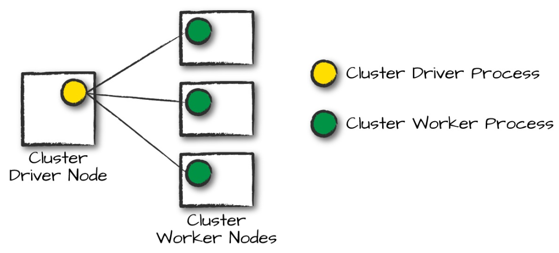
The Spark Driver
The driver is the process “in the driver seat” of your Spark Application. It is the controller of the execution of a Spark Application and maintains all of the state of the Spark cluster (the state and tasks of the executors). It must interface with the cluster manager in order to actually get physical resources and launch executors. At the end of the day, this is just a process on a physical machine that is responsible for maintaining the state of the application running on the cluster.
The Spark Executor
Spark executors are the processes that perform the tasks assigned by the Spark driver. Executors have one core responsibility: take the tasks assigned by the driver, run them, and report back their state (success or failure) and results. Each Spark Application has its own separate executor processes
The Cluster Manager
The Spark Driver and Executors do not exist in a void, and this is where the cluster manager comes in. The cluster manager is responsible for maintaining a cluster of machines that will run your Spark Application(s). Somewhat confusingly, a cluster manager will have its own “driver” (sometimes called master) and “worker” abstractions. The core difference is that these are tied to physical machines rather than processes (as they are in Spark). When it comes time to actually run a Spark Application, we request resources from the cluster manager to run it. Depending on how our application is configured, this can include a place to run the Spark driver or might be just resources for the executors for our Spark Application. Over the course of Spark Application execution, the cluster manager will be responsible for managing the underlying machines that our application is running on. In the following diagram, circles represent daemon processes running on and managing each of the individual worker nodes. There is no Spark Application running as of yet—these are just the processes from the cluster manager.
Spark currently supports three cluster managers: a simple built-in standalone cluster manager, Apache Mesos, Kubernetes, and Hadoop YARN. But be on the lookout in documentation as this list expands.
What are Execution Modes?
An execution mode gives you the power to determine where the aforementioned resources are physically located when you go to run your application. You have 3 options here:
Cluster mode:
Cluster mode is probably the most common way of running Spark Applications. In cluster mode, a user submits a pre-compiled JAR, Python script, or R script to a cluster manager. The cluster manager then launches the driver process on a worker node inside the cluster, in addition to the executor processes. This means that the cluster manager is responsible for maintaining all Spark Application–related processes.
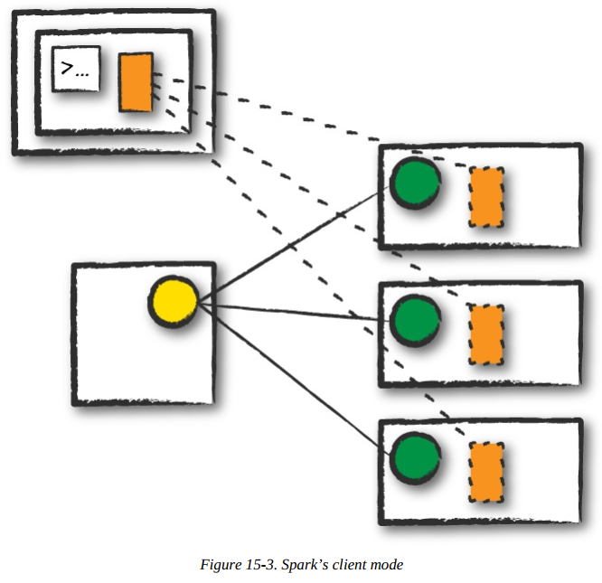
Client mode:
Client mode is nearly the same as cluster mode except that the Spark driver remains on the client machine that submitted the application. This means that the client machine is responsible for maintaining the Spark driver process, and the cluster manager maintains the executor processes. In figure, we are running the Spark Application from a machine that is not collocated on the cluster. These machines are commonly referred to as gateway machines or edge nodes. In figure you can see that the driver is running on a machine outside of the cluster but that the workers are located on machines in the cluster.
Local mode:
Local mode is a significant departure from the previous two modes: it runs the entire Spark Application on a single machine. It achieves parallelism through threads on that single machine. This is a common way to learn Spark, to test your applications, or experiment iteratively with local development. However, we do not recommend using local mode for running production applications.
./bin/spark-submit \
--class <main-class> \
--master <master-url> \
--deploy-mode cluster \
--conf <key>=<value> \
... # other options
<application-jar> \
[application-arguments]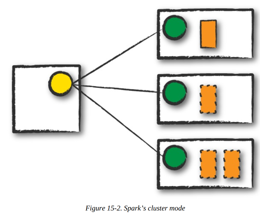
Driver
Driver
The Life Cycle of a Spark Application (Outside Spark)
Spark makes it easy to develop and create big data programs. Spark also makes it easy to turn your interactive exploration into production applications with spark-submit, a built-in command-line tool. spark-submit does one thing: it lets you send your application code to a cluster and launch it to execute there. Upon submission, the application will run until it exits (completes the task) or encounters an error. You can do this with all of Spark’s support cluster managers including Standalone, Mesos, and YARN. spark-submit offers several controls with which you can specify the resources your application needs as well as how it should be run and its command-line arguments. You can write applications in any of Spark’s supported languages and then submit them for execution. The simplest example is running an application on your local machine. We can also run a Python version of the application using the following command:
./bin/spark-submit \--master local \
./examples/src/main/python/pi.py 10
By changing the master argument of spark-submit, we can also submit the same application to a cluster running Spark’s standalone cluster manager, Mesos or YARN.
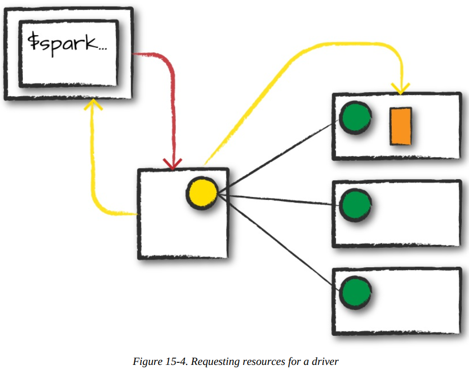
Client Request
The first step is for you to submit an actual application. This will be a pre-compiled JAR or library. At this point, you are executing code on your local machine and you’re going to make a request to the cluster manager driver node (refer figure). Here, we are explicitly asking for resources for the Spark driver process only. We assume that the cluster manager accepts this offer and places the driver onto a node in the cluster. The client process that submitted the original job exits and the application is off and running on the cluster. To do this, you’ll run something like the following command in your terminal:
Driver
Launch
Now that the driver process has been placed on the cluster, it begins running user code (refer diagram). This code must include a SparkSession that initializes a Spark cluster (e.g., driver + executors). The SparkSession will subsequently communicate with the cluster manager (the darker line), asking it to launch Spark executor processes across the cluster (the lighter lines). The number of executors and their relevant configurations are set by the user via the command-line arguments in the original spark-submit call. The cluster manager responds by launching the executor processes (assuming all goes well) and sends the relevant information about their locations to the driver process. After everything is hooked up correctly, we have a “Spark Cluster” as you likely think of it today.
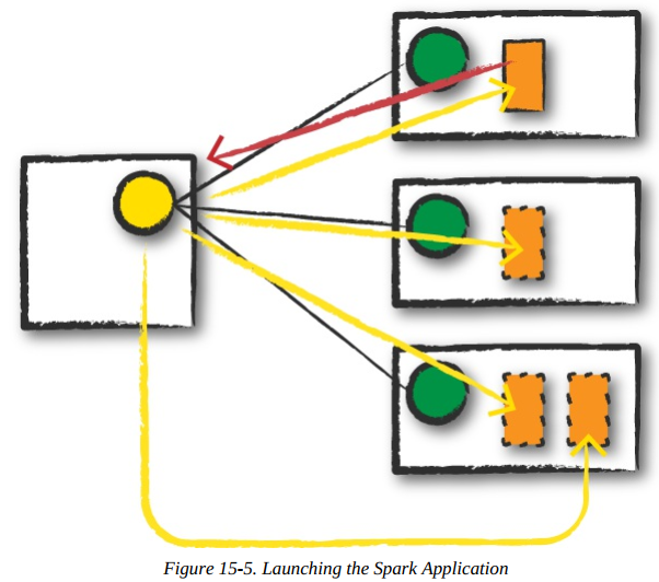
Driver
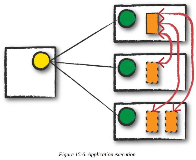
Execution
Now that we have a “Spark Cluster,” Spark goes about its merry way executing code, as shown in figure. The driver and the workers communicate among themselves, executing code and moving data around. The driver schedules tasks onto each worker, and each worker responds with the status of those tasks and success or failure.
Completion
After a Spark Application completes, the driver processes exits with either success or failure. The cluster manager then shuts down the executors in that Spark cluster for the driver. At this point, you can see the success or failure of the Spark Application by asking the cluster manager for this information.
Driver
The SparkSession
The first step of any Spark Application is creating a SparkSession. In many interactive modes, this is done for you, but in an application, you must do it manually. Some of your legacy code might use the new SparkContext pattern. This should be avoided in favor of the builder method on the SparkSession, which more robustly instantiates the Spark and SQL Contexts and ensures that there is no context conflict, given that there might be multiple libraries trying to create a session in the same Spark Application. After you have a SparkSession, you should be able to run your Spark code. From the SparkSession, you can access all of low-level and legacy contexts and configurations accordingly, as well. Note that the SparkSession class was only added in Spark 2.X. Older code you might find would instead directly create a SparkContext and a SQLContext for the structured APIs.
The Life Cycle of a Spark Application (Inside Spark) - The Important Stuff
This was life cycle of a Spark Application outside of user code, that is, the infrastructure that supports Spark. Now we talk about what happens within Spark when you run an application. This is the actual code that you write that defines your Spark Application i.e., user code. Each application is made up of one or more Spark jobs. Spark jobs within an application are executed serially (unless you use threading to launch multiple actions in parallel)
# Creating a SparkSession in Python
from pyspark.sql import SparkSession
spark = SparkSession.builder.master("local").appName("Word Count")\
.config("spark.some.config.option", "some-value")\
.getOrCreate()
The SparkContext
A SparkContext object within the SparkSession represents the connection to the Spark cluster. This class is how you communicate with some of Spark’s lower-level APIs, such as RDDs. It is commonly stored as the variable sc in older examples and documentation. Through a SparkContext, you can create RDDs, accumulators, and broadcast variables, and you can run code on the cluster. For the most part, you should not need to explicitly initialize a SparkContext; you should just be able to access it through the SparkSession.
After you initialize your SparkSession, it’s time to execute some code. As we know all Spark code compiles down to RDDs. Let’s walk through some DataFrame code, step by step to see what happens.
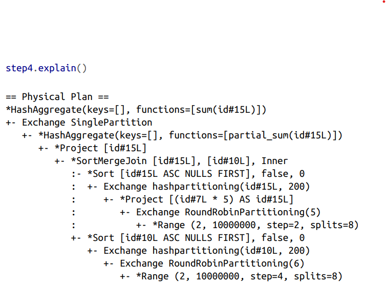
When you run this code, we can see that your action triggers one complete Spark job. Let’s take a look above at the explain plan to ground our understanding of the physical execution plan. We can access this information on the SQL tab (after we actually run a query) in the Spark UI, as well.
What you have when you call collect (or any action) is the execution of a Spark job that individually consist of stages and tasks. Go to localhost:4040 if you are running this on your local machine to see the Spark UI. We will follow along on the “jobs” tab eventually jumping to stages and tasks as we proceed to further levels of detail.
A Spark Job
In general, there should be one Spark job for one action. Actions always return results. Each job breaks down into a series of stages, the number of which depends on how many shuffle operations need to take place. This job breaks down into the following stages and tasks:
Stage 1 with 8 Tasks
Stage 2 with 8 Tasks
Stage 3 with 6 Tasks
Stage 4 with 5 Tasks
Stage 5 with 200 Tasks
Stage 6 with 1 Task
Stages
Stages in Spark represent groups of tasks that can be executed together to compute the same operation on multiple machines. In general, Spark will try to pack as much work as possible (i.e., as many transformations as possible inside your job) into the same stage, but the engine starts new stages after operations called shuffles. A shuffle represents a physical repartitioning of the data—for example, sorting a DataFrame, or grouping data that was loaded from a file by key (which requires sending records with the same key to the same node). This type of repartitioning requires coordinating across executors to move data around. Spark starts a new stage after each shuffle, and keeps track of what order the stages must run in to compute the final result.
In the job we looked at earlier, the first two stages correspond to the range that you perform in order to create your DataFrames. By default when you create a DataFrame with range, it has eight partitions. The next step is the repartitioning. This changes the number of partitions by shuffling the data. These DataFrames are shuffled into six partitions and five partitions, corresponding to the number of tasks in stages 3 and 4.
Stages 3 and 4 perform on each of those DataFrames and the end of the stage represents the join (a shuffle). Suddenly, we have 200 tasks. This is because of a Spark SQL configuration. The spark.sql.shuffle.partitions default value is 200, which means that when there is a shuffle performed during execution, it outputs 200 shuffle partitions by default. You can change this value, and the number of output partitions will change.
A good rule of thumb is that the number of partitions should be larger than the number of executors on your cluster, potentially by multiple factors depending on the workload. If you are running code on your local machine, it would behoove you to set this value lower because your local machine is unlikely to be able to execute that number of tasks in parallel. This is more of a default for a cluster in which there might be many more executor cores to use. Regardless of the number of partitions, that entire stage is computed in parallel. The final result aggregates those partitions individually, brings them all to a single partition before finally sending the final result to the driver.
Tasks
Stages in Spark consist of tasks. Each task corresponds to a combination of blocks of data and a set of transformations that will run on a single executor. If there is one big partition in our dataset, we will have one task. If there are 1,000 little partitions, we will have 1,000 tasks that can be executed in parallel. A task is just a unit of computation applied to a unit of data (the partition). Partitioning your data into a greater number of partitions means that more can be executed in parallel. This is not a panacea, but it is a simple place to begin with optimization.
Few more things to know about Execution details
Tasks and stages in Spark have some important properties that are worth reviewing. First, Spark automatically pipelines stages and tasks that can be done together, such as a map operation followed by another map operation. Second, for all shuffle operations, Spark writes the data to stable storage (e.g., disk), and can reuse it across multiple jobs.
Pipelining
An important part of what makes Spark an “in-memory computation tool” is that unlike the tools that came before it (e.g., MapReduce), Spark performs as many steps as it can at one point in time before writing data to memory or disk. One of the key optimizations that Spark performs is pipelining, which occurs at and below the RDD level. With pipelining, any sequence of operations that feed data directly into each other, without needing to move it across nodes, is collapsed into a single stage of tasks that do all the operations together. For example, if you write an RDD-based program that does a map, then a filter, then another map, these will result in a single stage of tasks that immediately read each input record, pass it through the first map, pass it through the filter, and pass it through the last map function if needed. This pipelined version of the computation is much faster than writing the intermediate results to memory or disk after each step. The same kind of pipelining happens for a DataFrame or SQL computation that does a select, filter, and select.
Shuffle Persistence
The second property you’ll sometimes see is shuffle persistence. When Spark needs to run an operation that has to move data across nodes, such as a reduce-by-key operation (where input data for each key needs to first be brought together from many nodes), the engine can’t perform pipelining anymore, and instead it performs a cross-network shuffle. Spark always executes shuffles by first having the “source” tasks (those sending data) write shuffle files to their local disks during their execution stage. Then, the stage that does the grouping and reduction launches and runs tasks that fetch their corresponding records from each shuffle file and performs that computation (e.g., fetches and processes the data for a specific range of keys). Saving the shuffle files to disk lets Spark run this stage later in time than the source stage (e.g., if there are not enough executors to run both at the same time), and also lets the engine re-launch reduce tasks on failure without rerunning all the input tasks. One side effect you’ll see for shuffle persistence is that running a new job over data that’s already been shuffled does not rerun the “source” side of the shuffle. Because the shuffle files were already written to disk earlier, Spark knows that it can use them to run the later stages of the job, and it need not redo the earlier ones. In the Spark UI and logs, you will see the pre-shuffle stages marked as “skipped”. This automatic optimization can save time in a workload that runs multiple jobs over the same data, but of course, for even better performance you can perform your own caching with the DataFrame or RDD cache method, which lets you control exactly which data is saved and where.
Conclusions
we discussed what happens to Spark Applications when we go to execute them on a cluster. This means how the cluster will actually go about running that code as well as what happens within Spark Applications during the process. At this point, you should feel quite comfortable understanding what happens within and outside of a Spark Application.
Logical Instructions
Spark code essentially consists of transformations and actions. How you build these is up to you—whether it’s through SQL, low-level RDD manipulation, or machine learning algorithms. Understanding how we take declarative instructions like DataFrames and convert them into physical execution plans is an important step to understanding how Spark runs on a cluster.
Logical instructions to physical execution
Let’s walk through a simple code that is doing a 3-step job: using a simple DataFrame, we’ll repartition it, perform a value-by-value manipulation, and then aggregate some values and collect the result.
# in Python
df1 = spark.range(2, 10000000, 2)
df2 = spark.range(2, 10000000, 4)
step1 = df1.repartition(5)
step12 = df2.repartition(6)
step2 = step1.selectExpr("id * 5 as id")
step3 = step2.join(step12, ["id"])
step4 = step3.selectExpr("sum(id)")
step4.collect() # 2500000000000